摘要:
介绍了K近邻算法,记录了MindSporeAI框架使用部分wine数据集进行KNN实验的步聚和方法。包括环境准备、下载红酒数据集、加载数据和预处理、搭建模型、进行预测等。
一、KNN概念
1. K近邻算法K-Nearest-Neighbor(KNN)
用于分类和回归的非参数统计方法
Cover、Hart于1968年提出
机器学习最基础的算法之一。
确定样本类别
计算样本与所有训练样本的距离
找出最接近的k个样本
统计样本类别
投票
结果就是票数最多的类。
三个基本要素:
K值,样本分类由K个邻居的“多数表决”确定
K值太小容易产生噪声
K值太大类别界限模糊
距离度量,特征空间中两个样本间的相似度
距离越小越相似
Lp距离(p=2时,即为欧式距离)
曼哈顿距离
海明距离
分类决策规则
多数表决
基于距离加权的多数表决(权值与距离成反比)
2.预测算法(分类)的流程
(1)找出距离目标样本x_test最近的k个训练样本,保存至集合N中;
(2)统计集合N中各类样本个数 Ci,i=1,2,3,...,c;
(3)最终分类结果为Ci最大的那个类(argmaxCi)。
k取值重要。
根据问题和数据特点来确定。
带权重的k近邻算法
每个样本有不同的投票权重
3.回归预测
回归预测输出为所有邻居的标签均值:
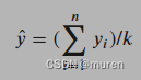
yi为k个目标邻居样本的标签值
带样本权重的回归预测函数:
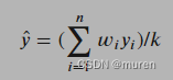
ωi为第个i样本的权重
4. 距离的定义
常用欧氏距离(欧几里得距离)
空间中两点x和y之间的欧氏距离公式:
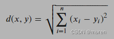
注意将特征向量的每个分量归一化
减少不同尺度的干扰
大数值特征分量会淹没小数值特征分量
其它距离
Mahalanobis距离
Bhattacharyya距离
二、环境配置
%%capture captured_output
# 实验环境已经预装了mindspore==2.2.14,如需更换mindspore版本,可更改下面mindspore的版本号
!pip uninstall mindspore -y
!pip install -i https://pypi.mirrors.ustc.edu.cn/simple mindspore==2.2.14
# 查看当前 mindspore 版本
!pip show mindspore
输出:
Name: mindspore
Version: 2.2.14
Summary: MindSpore is a new open source deep learning training/inference framework that could be used for mobile, edge and cloud scenarios.
Home-page: https://www.mindspore.cn
Author: The MindSpore Authors
Author-email: contact@mindspore.cn
License: Apache 2.0
Location: /home/nginx/miniconda/envs/jupyter/lib/python3.9/site-packages
Requires: asttokens, astunparse, numpy, packaging, pillow, protobuf, psutil, scipy
Required-by: mindnlp
三、下载红酒数据集
1. Wine数据集
官网链接:UCI Machine Learning Repository
http://archive.ics.uci.edu/dataset/109/wine
数据内容:
意大利同一地区、三个不同品种葡萄酒化学分析结果。
包括每种葡萄酒中所含13种成分的量:
| Alcohol | 酒精 |
| Malic acid | 苹果酸 |
| Ash | 灰 |
| Alcalinity of ash | 灰的碱度 |
| Magnesium | 镁 |
| Total phenols | 总酚 |
| Flavanoids | 类黄酮 |
| Nonflavanoid phenols | 非黄酮酚 |
| Proanthocyanins | 原花青素 |
| Color intensity | 色彩强度 |
| Hue | 色调 |
| OD280/OD315 of diluted wines | 稀释酒的OD280/OD315 |
| Proline | 脯氨酸 |
方式一,从Wine数据集官网下载wine.data文件。
方式二,从华为云OBS中下载wine.data文件。
| Key | Value | Key | Value |
| Data Set Characteristics | Multivariate | Number of Instances | 178 |
| Attribute Characteristics | Integer, Real | Number of Attributes | 13 |
| Associated Tasks | Classification | Missing Values? | No |
2.下载数据集
from download import download
# 下载红酒数据集
url = "https://ascend-professional-construction-dataset.obs.cn-north-4.myhuaweicloud.com:443/MachineLearning/wine.zip"
path = download(url, "./", kind="zip", replace=True)输出:
Downloading data from https://ascend-professional-construction-dataset.obs.cn-north-4.myhuaweicloud.com:443/MachineLearning/wine.zip (4 kB)

file_sizes: 100%|██████████████████████████| 4.09k/4.09k [00:00<00:00, 2.35MB/s]
Extracting zip file...
Successfully downloaded / unzipped to ./
四、数据读取与处理
1.加载数据
导入os、numpy、MindSpore、matplotlib等模块
用context.set_context()配置运行模式、后端信息、硬件等
读取Wine数据集wine.data
查看部分数据。
%matplotlib inline
import os
import csv
import numpy as np
import matplotlib.pyplot as plt
import mindspore as ms
from mindspore import nn, ops
ms.set_context(device_target="CPU")
with open('wine.data') as csv_file:
data = list(csv.reader(csv_file, delimiter=','))
print(data[56:62]+data[130:133])输出:
[['1', '14.22', '1.7', '2.3', '16.3', '118', '3.2', '3', '.26', '2.03', '6.38', '.94', '3.31', '970'],
 ['1', '13.29', '1.97', '2.68', '16.8', '102', '3', '3.23', '.31', '1.66', '6', '1.07', '2.84', '1270'],
 ['1', '13.72', '1.43', '2.5', '16.7', '108', '3.4', '3.67', '.19', '2.04', '6.8', '.89', '2.87', '1285'],
 ['2', '12.37', '.94', '1.36', '10.6', '88', '1.98', '.57', '.28', '.42', '1.95', '1.05', '1.82', '520'],
 ['2', '12.33', '1.1', '2.28', '16', '101', '2.05', '1.09', '.63', '.41', '3.27', '1.25', '1.67', '680'],
 ['2', '12.64', '1.36', '2.02', '16.8', '100', '2.02', '1.41', '.53', '.62', '5.75', '.98', '1.59', '450'],
 ['3', '12.86', '1.35', '2.32', '18', '122', '1.51', '1.25', '.21', '.94', '4.1', '.76', '1.29', '630'],
 ['3', '12.88', '2.99', '2.4', '20', '104', '1.3', '1.22', '.24', '.83', '5.4', '.74', '1.42', '530'],
 ['3', '12.81', '2.31', '2.4', '24', '98', '1.15', '1.09', '.27', '.83', '5.7', '.66', '1.36', '560']]
三类样本(共178条)
自变量X为数据集的13个属性
因变量Y为数据集的3个类别
取样本的某两个属性进行2维可视化
可以看到在某两个属性上样本的分布情况以及可分性。
X = np.array([[float(x) for x in s[1:]] for s in data[:178]], np.float32)
Y = np.array([s[0] for s in data[:178]], np.int32)
attrs = ['Alcohol', 'Malic acid', 'Ash', 'Alcalinity of ash', 'Magnesium', 'Total phenols',
         'Flavanoids', 'Nonflavanoid phenols', 'Proanthocyanins', 'Color intensity', 'Hue',
         'OD280/OD315 of diluted wines', 'Proline']
plt.figure(figsize=(10, 8))
for i in range(0, 4):
    plt.subplot(2, 2, i+1)
    a1, a2 = 2 * i, 2 * i + 1
    plt.scatter(X[:59, a1], X[:59, a2], label='1')
    plt.scatter(X[59:130, a1], X[59:130, a2], label='2')
    plt.scatter(X[130:, a1], X[130:, a2], label='3')
    plt.xlabel(attrs[a1])
    plt.ylabel(attrs[a2])
    plt.legend()
plt.show()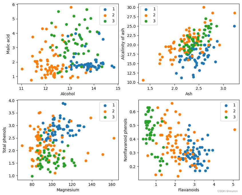
2.数据预处理
将数据集按128:50划分为训练集(已知类别样本)和验证集(待验证样本):
train_idx = np.random.choice(178, 128, replace=False)
test_idx = np.array(list(set(range(178)) - set(train_idx)))
X_train, Y_train = X[train_idx], Y[train_idx]
X_test, Y_test = X[test_idx], Y[test_idx]五、模型构建--计算距离
MindSpore算子
tile
square
ReduceSum
sqrt
TopK
矩阵运算并行计算
目标样本x和已分类训练样本X_train的距离
top k近邻
class KnnNet(nn.Cell):
def __init__(self, k):
super(KnnNet, self).__init__()
self.k = k
def construct(self, x, X_train):
#平铺输入x以匹配X_train中的样本数
x_tile = ops.tile(x, (128, 1))
square_diff = ops.square(x_tile - X_train)
square_dist = ops.sum(square_diff, 1)
dist = ops.sqrt(square_dist)
#-dist表示值越大,样本就越接近
values, indices = ops.topk(-dist, self.k)
return indices
def knn(knn_net, x, X_train, Y_train):
x, X_train = ms.Tensor(x), ms.Tensor(X_train)
indices = knn_net(x, X_train)
topk_cls = [0]*len(indices.asnumpy())
for idx in indices.asnumpy():
topk_cls[Y_train[idx]] += 1
cls = np.argmax(topk_cls)
return cls六、模型预测
验证KNN算法
k=5
验证精度接近80%
acc = 0
knn_net = KnnNet(5)
for x, y in zip(X_test, Y_test):
    pred = knn(knn_net, x, X_train, Y_train)
    acc += (pred == y)
    print('label: %d, prediction: %s' % (y, pred))
print('Validation accuracy is %f' % (acc/len(Y_test)))
输出:
label: 1, prediction: 1
label: 3, prediction: 3
label: 3, prediction: 3
label: 3, prediction: 3
label: 3, prediction: 3
label: 3, prediction: 3
label: 1, prediction: 1
label: 3, prediction: 1
label: 1, prediction: 1
label: 1, prediction: 2
label: 3, prediction: 3
label: 1, prediction: 1
label: 3, prediction: 3
label: 1, prediction: 1
label: 1, prediction: 1
label: 3, prediction: 2
label: 1, prediction: 1
label: 3, prediction: 3
label: 1, prediction: 1
label: 1, prediction: 3
label: 1, prediction: 1
label: 1, prediction: 1
label: 1, prediction: 3
label: 1, prediction: 1
label: 3, prediction: 2
label: 1, prediction: 1
label: 3, prediction: 2
label: 3, prediction: 2
label: 1, prediction: 1
label: 3, prediction: 1
label: 3, prediction: 1
label: 1, prediction: 1
label: 2, prediction: 3
label: 2, prediction: 2
label: 2, prediction: 2
label: 2, prediction: 2
label: 2, prediction: 2
label: 2, prediction: 2
label: 2, prediction: 3
label: 2, prediction: 2
label: 2, prediction: 3
label: 2, prediction: 2
label: 2, prediction: 2
label: 2, prediction: 2
label: 2, prediction: 3
label: 2, prediction: 2
label: 2, prediction: 2
label: 2, prediction: 2
label: 2, prediction: 2
label: 2, prediction: 2
Validation accuracy is 0.720000